How much carbon dioxide can we emit?

Mother Earth is warming, and the piling up of CO₂ in the atmosphere is to blame:

One of the key headlines from the Synthesis Report of the Intergovernmental Panel on Climate Change’s (IPCC's) Fifth Assessment Report was: “Cumulative emissions of CO₂ largely determine global mean surface warming by the late 21st century and beyond.”

The Carbon Budget, for dummies

Carbon Budget. The concept is beautiful! Given a goal of not exceeding 2°C, and how much we’ve already emitted, we can calculate the actual amount of CO₂ – the ‘carbon budget’ – that is left to us.

The Synthesis Report said that a remaining carbon budget of about 1000 billion tonnes CO₂ to be emitted from 2012 onwards would limit total human-induced warming to less than 2°C relative to the period 1861–1880 with a probability of greater than 66% (a likely chance in the IPCC lingo).

With current emissions levels of 40 billion tonnes CO₂ per year, this remaining carbon budget has already dropped since 2012 to about 800GtCO₂, and if emissions continue at today’s level, the budget will be entirely gone in just 20 years.

IPCC's Report continues: “Estimated total fossil carbon reserves exceed this remaining amount by a factor of 4 to 7, with resources much larger still”.

The implications are clear: time is short and we cannot use all known fossil fuel reserves.

In fact, the whole cumulative emissions concept opened a new political discussion. “Keep it in the ground”, “unburnable carbon”, and “stranded assets” are now common terms in climate policy discussions.

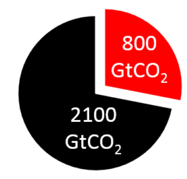
Carbon budget insights: 1;We have already emitted 2100 billion tonnes CO₂, and if we emit 800 billion tonnes more, then there is a 66% chance we will stay below 2°C. 2; We will have emitted this CO₂ by about 2040 at current emission rates. 3; A beautifully simple concept, but one that is far more complex in reality.

Hold your horses, it is not so simple!

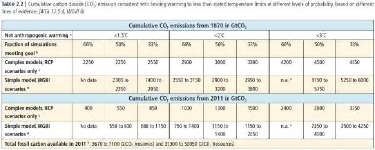
The budget is so simple, it should be easy to update with each new year of emissions, so we can track how fast the carbon budget ‘pie’ is getting eaten. Right? The problem is that there is no ‘unique’ carbon budget, but many equally defendable carbon budgets (Figure 2).

To work through the multiple carbon budgets, I will discuss four choices one must make when choosing a budget:

1. Temperature and Probability: The remaining carbon budget concept is probabilistic, due to the uncertainties in the climate system, and the IPCC gives remaining carbon budgets with a probability of 33%, 50%, and 66% of staying below 1.5°C, 2°C, and 3°C.

2. Type of model: The IPCC presented two different budgets from ‘complex models’ and ‘simple models’. The budget for 2°C and a 66% probability, we could choose the 1000 billion tonnes CO₂ remaining carbon budget (‘complex models’ from 2011) or the range of 750 to 1400 billion tonnes CO₂ (‘simple models’ from 2011).

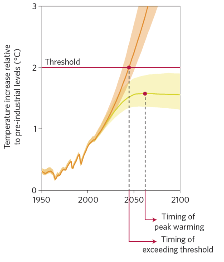
3. Definitions: The IPCC used, without being specific, three different definitions: the “Threshold Exceedance Budget”, “Threshold Avoidance Budget”, and cumulative emissions between 2010 and 2050, and 2010 and 2100. As it happens, the ‘complex models’ use an Exceedance Budget and the ‘simple models’ use an Avoidance Budget.

4. Year: The IPCC gives carbon budgets ‘from 1870’ and ‘from 2011’. One would think they only differ by the estimated historical cumulative CO₂ emissions. Well, it is a touch more complex.

On top of this, there are structural and parametric uncertainties in modelling the climate and socio-economic system, and uncertainty in the estimates of historical emissions. For now, let’s put those uncertainties aside and focus on definitions.

What choices should I make?

As should be clear by now, and to the disappointment of everyone, there is no single magic remaining carbon budget. There are too many value-based choices, modelling choices, and uncertainties to determine a single number.

The choice on temperature and probability is, relatively speaking, straightforward. The IPCC generally refers to 2°C with a 66% chance, arguably somewhat consistent with the “well below 2°C” mentioned in the Paris Agreement. The International Energy Agency’s (IEA) 450 scenario is consistent with 2°C and a 50% chance. As for now, let’s work with 2°C with a 66% chance.

Our next step: The choice between ‘complex model’ and ‘simple model’ is more complex, and requires a longer discussion.

To avoid or to exceed, that is the question

To help explain the differences between ‘complex models’ and ‘simple models’, let us take a detour into the models and how they work.

Complex models:

The ‘complex models’ are Earth System Models (ESMs) and Earth System Models of Intermediate Complexity (EMICs) used to estimate “Threshold Exceedance Budgets” using a high-end scenario (called RCP8.5). These are the models that describe the evolving climate in excruciating detail and run on supercomputers. The models have ‘internal variability’, just as the weather varies from day to day, and consequently they have to be run many times to get the ‘average’ climate (each set of runs is known as an ensemble).

For each model and ensemble, the cumulative CO₂ is estimated at the time the temperature “exceeds” a given temperature threshold. The outputs from multiple models and runs are collated, and the cumulative CO₂ emissions are estimated as when 33%, 50%, or 66% of the model-ensemble combinations exceed the given temperature level. The probability in the ‘complex models’ reflects the variation between models and not a systematic assessment of the uncertainties in the climate system.

Simple models:

The ‘simple models’ are Integrated Assessment Models (IAMs), and not really that simple! They are models of the socio-economic system, primarily the energy system, and are used to analyze mitigation pathways. The models output emissions pathways, from which temperature pathways can be estimated using a ‘simple climate model’ (a version of the ‘complex models’ which runs in a matter of seconds on a desktop computer).

A probabilistic temperature response can be estimated based on uncertainties in the climate system (33%, 50%, 66% probability), but this is a rather different uncertainty to what is used in the ‘complex models’ (let’s skip those details!). Because the models run relatively quickly, they can estimate the remaining carbon budget for multiple scenarios, as opposed to just one scenario for the complex models. The carbon budget, then, is calculated from the cumulative CO₂ emissions when the temperature peaks for all scenarios that stay below the limit (e.g. 2°C).

Since the ‘simple models’ use a range of scenarios, each with a unique non-CO₂ emission pathway, they result in a range of carbon budgets! The probability in the ‘simple models’ reflects a comprehensive assessment of the uncertainties in the climate system, albeit using a ‘simple climate model’.

As an aside, for those that are curious, it is also possible to estimate cumulative CO₂ emissions for a given time-period, such as over the period 2011-2050 and 2011-2100.

In sum:

The ‘complex models’ use a single scenario and an ‘exceedance budget’ The ‘simple models’ use multiple scenarios and an ‘avoidance budget’

Generally, each scenario has a different non-CO₂ emission pathway, and hence multiple scenarios lead to multiple carbon budgets (hence the carbon budget range in the ‘simple model’ budgets).

The carbon budgets from the ‘complex models’ and ‘simple models’ are both correct, but report different information. It makes sense, therefore, to report both sets of numbers.

A rather technical, but nonetheless important, point is that the probability in the ‘complex models’ and ‘simple models’ is not directly comparable.

It is a carbon budget, so why is non-CO₂ important?

We emit a variety of greenhouse gases that affect the climate. CO₂ is the most dominant and longest living. It is not possible to solve the climate problem without solving the CO₂ problem. Mitigation of other greenhouse gases, such as methane and nitrous oxide, can lead to more rapid stabilization of temperatures and keep temperatures at a lower level.

In principle, the carbon budgets could be calculated for CO₂ emissions only. We emit other greenhouse gases that lead to temperature changes, and thus the CO₂-only-carbon-budgets need to be reduced to account for the non-CO₂ temperature contributions. (The impact of non-CO₂ emissions of carbon budgets will be the topic of another blog post.)

Historical emission estimates

There is a relatively accepted value for historical CO₂ emissions, despite uncertainties. However, the way the ‘complex models’ described above are used complicates matters.

We have two main ways to run the ‘complex models’:

• ‘concentration driven’ uses atmospheric concentrations as input,
• ‘emission driven’ uses greenhouse gas emissions as input.

The major difference between the two are biogeochemical cycles (carbon, methane, etc). The carbon cycle is one of the biggest uncertainties in the climate system, and a ‘concentration driven’ calculation allows focus on the climate system without including the complexities of the carbon cycle or atmospheric chemistry.

It is possible to estimate emissions from a complex model in ‘concentration driven’ mode, by doing an ‘inverse’ (backwards) calculation. Since the carbon cycle is one of the most uncertain parts of the climate system, each complex model can have rather different estimates of historical emissions. This is clear from Figure 2, where subtracting the cumulative emissions ‘from 1870’ and ‘from 2011’ for the complex models gives implied historical emissions of 1600 billion tonnes CO₂ to 1900 billion tonnes CO₂.

dditionally, for some complex models, the historical emissions are for fossil fuel and industry only, requiring some assumptions about land-use change.

Put simply: the historical emissions from the complex models are much more uncertain then the historical emissions we measure.

The ‘simple models’ do not have this problem, and all rows in the IPCC’s summary table (Figure 2) give cumulative CO₂ emissions from 1870 to 2011 of 1750 billion tonnes CO₂.

However, our knowledge of historical emissions has changed in the last few years, and the latest estimated emissions from 1870-2011 are now 1884 billion tonnes CO₂, about 100 billion tonnes CO₂ larger than reported by the IPCC over the same time-period in 2014.

Over the period 2012-2016, emissions of about 200 billion tonnes CO₂ have occurred.

Total emissions from 1870-2016 are 2080 billion tonnes CO₂.

I want the latest carbon budget, from the IPCC, how do I estimate it?

The IPCC estimates two different budgets for two different time periods (Figure 2).

I would recommend using the carbon budgets from both the ‘complex models’ and ‘simple models’. Use the ‘complex model’ estimate as a central estimate, and the ‘simple model’ estimates as a range.

Due to the complexities and revisions in historical emissions, I recommend using the ‘from 1870’ cumulative CO₂ emissions, and subtracting the latest estimates of historical CO₂ emissions since then.

For a 2°C with a 66% chance, this would give 800 billion tonnes CO₂ for the ‘complex models’ and 450-1050 billion tonnes CO₂ for the ‘simple models’. All these numbers are rounded to the nearest 50 billion tonnes CO₂.

Complexities with 1.5°C

There is now a lot of interest in the 1.5°C carbon budget, particularly since the Paris Agreement.

The remaining carbon budget for 1.5°C from the ‘complex models’ varies depending on assumptions. For a 50% chance at 1.5°C the updated budget derived ‘from 1870’ is 150 billion tonnes CO₂ (2250 – 2100), but updated ‘from 2011’ is 350 billion tonnes CO₂ (550 – 200).

The updated remaining carbon budget from the ‘simple models’ is either 200-250 billion tonnes CO₂ (‘from 1870’) or 350-400 billion tonnes CO₂ (‘from 2011’). Neither of the ranges overlap with the value from the ‘complex models’, probably since the there are so few scenarios consistent with 1.5°C.

In both cases, the differences between the 'from 1870' and 'from 2011' budgets are due to differences in historical emission estimates. I would therefor recommend using the 'from 1870' budgets and deducting the most recent estimates of historical CO₂ emissions (2100 billion tonnes CO₂) to get the updated remaining carbon budget.

For a 1.5°C with a 50%-66% chance, I recommend 150 billion tonnes CO₂, but note the large uncertainty associated with this estimate.

The moral of the story

The moral of the story is that there is not a single “carbon budget”. However, the core message of the ‘carbon budget’ concept is that emissions need to go to net-zero (otherwise, the budget continues to grow).

Whether the remaining budget is 700, 800, or 900 billion tonnes CO₂ is largely beside the point. Due to the uncertainty in future non-CO₂ pathways, we simply do not know. Either way, emissions need to go to zero at an unprecedented rate.

Fossil fuels, according to the IPCC will need to stay on the ground, but the amount staying in the ground will depend on the carbon budget and negative emissions . A topic for a future blog post.

Våre prosjekter

• Global Carbon Project